The trap of OEE obsession

 Production obsession for OEE

Generations of production managers and directors have been trained to optimize the OEE of their equipment - all their equipments.
In their minds, a machine that doesn't run is a waste. So is an operator who doesn't produce parts.
So, historically, we've been inclined to make the most of existing resources, to invest in equipment as fairly as possible, to decide on an investment as late as possible, and to add teams only as late as possible - and often too late.
We can't blame our production managers: their managerial performance is probably indexed to OEE - and we behave according to how we're measured.

Utilization rate and ability to deliver  

The effect of these decisions on our ability to serve customers can be catastrophic. As we wait as long as possible to increase capacity, we wait until we are structurally behind schedule. Our chronic backlog shows management that we need to invest - but by the time the capacity increase is effective (it may take several months) - our backlog will get worse.
Some industries pay a high price for this way of thinking. The chronic difficulties of players in the aerospace and defense industries are a case in point.
The correlation between resource utilization and lead times - and the impact of variability - is poorly understood. 

"However, in our S&OP, our average projected load was lower than our installed capacity."

Ahah. This raises several questions:

-    Is an "average" load indicative of our requirements?
-    By how much should our load be less than capacity?
-    What is our actual installed capacity? 

Kingman's formula

Formulated in 1961, Kingman's formula approximates the waiting time for a resource as a function of its saturation rate. 
It can be used to evaluate queues (and therefore lead times in our supply chain).  

This article from AllAboutLean describes the lessons to be learned from this formula: https://www.allaboutlean.com/kingman-formula/
Two major factors affect lead times:

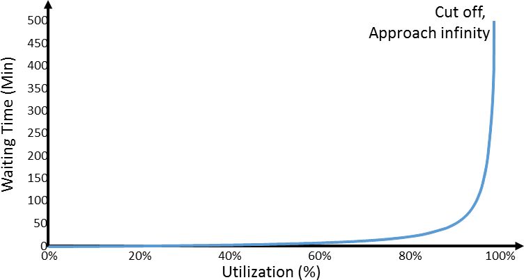
1.    Utilization rate. The closer you get to 100% utilization, the more your lead times tend... to infinity!

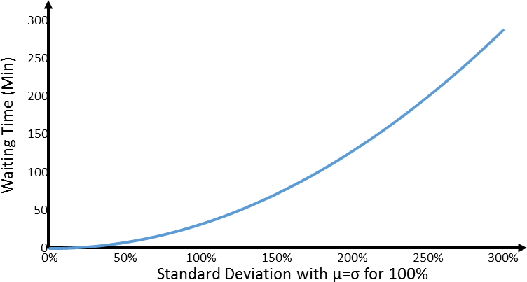
2. Variability. The greater the variability, the longer the delay.

Isn't this an interesting formula to explain to our production managers, as well as to the Finance community in our plants?

An example

Let's take the example of a supermarket checkout queue. This example was presented by Adnen Ben Sedrine from Safran at our latest user conference.

The average processing time for a cart is 2 minutes, and on average there are 20 customers per hour during the day. We have a capacity of 30 customers per hour, our utilization rate is 67%, so all's well!

Customer arrivals are random. C_a^2For example = 1.5
Cart processing time is also variable. C_s^2For example = 1

If you apply the formula :

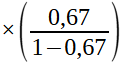
= at 20 customers/h, waiting time is 0,084h = 5’

  = at 27 customers/h, it becomes = 0,338h = 20’

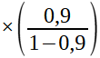
= at 29 customers/h, it becomes = 0,713h = 43' 43d’

How can you make the most of this formula?

Applied to production in your plant, we can draw a few lessons:

• OEE is only relevant to your actual capacity constraints, and its function is to help you reduce variability and increase throughput on these resources.
• Queues (time buffers) are powerful management tools for controlling priorities, monitoring work-in-progress and activating resources as required.
• In your S&OP, keep a safety margin of at least 15% in relation to your demonstrated capacity.
• Don't base your operating model on an average: integrate variability into your model.

Steering by constraints, optimizing efficiency, managing queues, projecting your S&OP on the basis of your demonstrated capacity and simulating the effect of variability - Intuiflow can help you take advantage of these best practices!