
Four years ago I was invited to introduce DDMRP to a team from a medical device company, a subsidiary of a German group. Supply chain, purchasing, production, quality were in the room. They wanted to know more because they were suffering from long lead times, too much stock, unsatisfactory service levels, and faced many emergencies.
The company had carried out several projects to improve the situation, and used up several supply chain managers. One of the key projects at the time was ” TCO ” : improve the “total cost of ownership”. I thought the initiative was a positive one: the company was sourcing many products from Asia to Europe, so taking into account the true total cost of ownership in sourcing decisions could only be a good thing.
My presentation was well received, until I got carried away with enthusiasm and cheerfully disparaged Wilson’s formula, the one we used years ago to calculate an economic order quantity, remember?
While I was heavily emphasizing the damage that this formula had done to the industry, I felt a growing discomfort with my audience.
After some awkward exchanges, it turned out that the famous “total cost of ownership” project consisted essentially of increasing the purchased batch sizes, so as to reduce the burden of entry quality control. Indeed, in pharma or medical devices, entry control is a key operation, which requires perfect batch traceability, and it can be a heavy operation.
Following a flow mapping, the team found that the biggest lead time at their site was the queue before entry control. From memory, the average was more than three weeks.
The conclusion they had drawn? In order to reduce lead times in the facility and cut costs, we need fewer batches to be controlled. To do this, we’re going to massively increase the quantity ordered on each batch by integrating the cost of entry control into Wilson’s formula, in addition it will allow us to place spot orders of big quantities with ad hoc suppliers.
OK, you see me coming, this goes a bit against supply chain flow, and against the real total cost of ownership.
We parted amicably after my presentation, and they did not call me back… A priority they are now starting to look again at DDMRP, perhaps the TCO project did not bring the expected gains.
Were there solutions to alleviate the capacity constraint of this entry control? The process was fully manual, with no electronic batch record, there was a lack of versatility of the teams, some measuring equipment was saturated and the ad hoc suppliers could not be under QA supplier agreements, which made the controls more cumbersome. So many avenues for progress, no doubt…
Let’s go back to today. We have just welcomed in our team a young student in Supply Chain Management. As I explained to him on Friday that Wilson’s formula was to be banned, he stared at me : he has been taught this formula for years to determine economic quantities, it was even the preferred topic of one of his professors!
Teaching the younger generation the Wilson formula in 2020 is a crime against the flow of the years to come, isn’t it?
Now, you tell me, why so much hatred against Wilson’s formula? After all, it sounds scientific, doesn’t it? It has a square root!
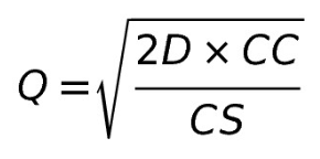
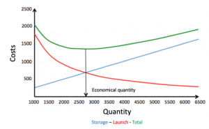
Wilson’s formula is a good example of a precise formula. We divide a numerator by a denominator, and take the square root. Established in 1934, it establishes the optimal point of total cost between the cost of holding inventory and the cost of placing an order. It Is indisputable.
A few small details:
How is the cost of ownership calculated? What is the cost of carrying inventory? What is the real cost of capital tied up in this stock? What is the cost of non-quality, storage, obsolescence? What is the cost of overstock? What is the cost of a shortage? What is the cost of lost sales? How do we calculate this cost without mixing variable and fixed costs ?
And the cost of placing an order, what is it? I’ve known companies that have made the following calculation: I have four suppliers, each one works 1600 hours a year, they process 10,000 orders a year, so I have a cost per order line of 0.64 hours of one supplier. Hmm – if I place 1000 orders less will I save 640 hours?
In summary: Wilson’s formula applies a square root to the ratio of one arbitrary guesstimate divided by another arbitrary guesstimate. This is a nice example of precisely wrong calculation, isn’t it?
This 1934 reasoning is clearly no longer applicable, if it ever was.
This formula has led the majority of companies to hinder their flow, whereas the core business of a company is to generate a fast and reliable flow of products that meet customer expectations!
It is not a matter of ignoring real constraints that induce costs. This is often a stumbling block in lean approaches: the “one-piece flow”, where batch size is 1 , is unrealistic in most cases.
A truck or container has a cost and an environmental footprint. Changeovers that take time on a fully loaded equipment have a cost. Material losses related to washing between two products in process industries have a cost.
Even if we can improve the flexibility of our production means with SMED approaches and technological evolutions, we must not ignore these costs, and we must take them into account in the design of our model.
The Demand Driven Model
The Demand Driven model provides us with valuable support in addressing the issue of batch sizes, and working to align them with the establishment of a fast and reliable material flow:
Shared visibility
The batch sizes of the stored positions are materialized by the green areas of the buffers. When these green areas are disproportionate to the red and yellow areas, it is obvious. If your buyers, your producers, your supply chain, technical teams, marketing have been trained to DDMRP, they all understand the same thing and the impact of the green zones. It becomes easier to align each other’s views.
Economic impact
The impact of the green zone on stock values is easy to translate into inventory levels. The operating model can be simulated with several lot sizes, and the impacts on inventory, service, lead times, number of series changes are easy to evaluate.
Pragmatism of batch sizes
The use of order cycles (interval in days between each lot), or a lead time factor (use of a percentage to establish a reasonable lot size in relation to a short, medium or long lead time) allow to size a model compatible with existing constraints.
Group planning
The stock buffers and DDMRP time buffers easily allow group planning : grouping together like items that can be batched together at a lower cost, while taking into account customer priorities in real time. This is a very efficient way to reduce lot sizes at SKU level without deteriorating costs. The definition of these rules in the design of the operational model allows to ask the right questions and to extract from the head of the operational or from the meander of Excel files the logic adapted to manage a given flow.
Continuous Improvement
The performance of the Demand Driven model is continuously measured, levers for improvement are highlighted, and teams are encouraged to continuously improve the model.
What is an economical lot size eventually ? A batch that enables quick material flow, that is compatible with the current state of our capabilities, that takes into account our constraints in a pragmatic way, and that we will work constantly to reduce. It does not need a square root equation, but it requires the knowledge and collective intelligence of our teams!
If you are interested in learning more about our Demand Driven Supply Chain Software solutions feel free to contact us and see how DDMRP can improve your supply chain.