There are many ways to calculate the optimal production batch. In this article, we’ll review several different formulas — and discuss a related indicator, the production order cycle, which addresses how often each SKU should be placed into production. The goal? To find a method that balances business assets with current market needs, rather than minimum unit cost.
That’s because — as George Possel said — all benefits are directly related to the speed of flow of relevant information and materials. A secure, balanced flow of relevant information and materials increases service levels. When you get and pass the correct signals along your supply chain at the right time, you ensure that items you need are always in the right place. This leads to an increase in sales, a reduction in overstocks, and thus an increase in return on investment (ROI). Unit cost does not figure here; flow is the only thing that matters.
The Basics of Production Cycles
Traditionally, production units strive to make their production cycles, like their batches, as large as possible. Thus, the time for changeovers decreases and the utilization rate of the equipment increases. Let’s say, for example, the changeover time is 3 hours. One changeover per day is 12.5% downtime. One changeover per week means less than 2% downtime. In addition, due to economies of scale, there is often a reduction in unit cost.
But such production indicators have their price. Production cycles that are too long lead to:
- Overstocks and additional costs
- A shortage of raw materials and semi-finished parts (if, for example, we produce two SKUs from one raw material)
- A shortage of production capacity (if we don’t have time to produce everything in large quantities)
On the other hand, we have the lean manufacturing approach, which considers stock among the system as a waste. And in an ideal system, there should be no limit to the minimum batch, i.e., production can release one piece. In reality, the less the better, depending on takt time. And it is desirable to order and not to stock (Kanban, Just in time). At the same time, in order not to lose in efficiency, these approaches have tools to reduce changeover time.
This approach is good at the operational level and in a world where there is no significant demand variability. In reality, this will lead to an increased whiplash. Market variability will be directly passed into the system. The chance of failure will increase. In addition, it has no connection with our broader business strategy — the decision to enter new markets or make changes to assortment matrices mean we have to rebuild this fragile model too often.
In an attempt to find a balance, several techniques have been created. For example, one of the most popular, EOQ (economic order quantity), calculates the batch based on the cost of ordering, receiving, and storing the order. However, it has its own conditions, or assumptions:
- The demand is known
- The Lead time is known and constant
- The goods are received instantly
- The model does not take into account wholesale prices
- Out of stock is not allowed
In today’s world, demand is volatile and unpredictable, as is supply. As a result, there may be out of stock. And instant receipt of the goods is impossible. Meaning that we cannot fulfill four out of five conditions that are necessary for the successful application of this model.
Using DDMRP to Balance Business Assets
In the DDMRP methodology, the order size and frequency are determined by the green zone of Demand Driven buffers.
On the one hand, this incorporates real logistical restrictions, such as the minimum possible production batch (minimum order quantity) and the order cycle both for production or ordering a supplier. On the other hand, if there are no such restrictions, or they are not enough to protect the system from external variability, there is a calculated value of the green zone. It should also be noted that the order cycle is in some cases a constraint and in some cases a control lever. DDMRP makes it possible to calculate the production cycle in such a way as to be as flexible as possible in relation to market demand within the possible allowable number of changeovers.
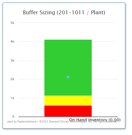
On the one hand, this technique enables you not to freeze extra money in stock. On the other hand, it protects your supply chain from external variability. The green buffer zone absorbs demand variability. This allows you to protect your system from market fluctuations and frequent changeovers. It also facilitates the transfer of aggregated orders further down the supply chain with a more stable volume and frequency.