Even today, we encounter companies that have difficulty differentiating their stocking strategies according to demand profiles. Have you ever been instructed to put a month’s worth of stock on hand to secure sales?
In several industrial and distribution sectors, this policy is simply based on ensuring a certain number of days of coverage, and it’s not differentiated by product.
One month you can sell 10,000 and the next month 5,000. How much is a month’s supply?
“One month’s worth of inventory,” of course, means nothing. It means something after the fact, when you’re tracking the performance of your inventory turns — but it’s not relevant to sizing your replenishment loops.
Statistical Formulas and Variability Factors
For decades, people have proposed statistical formulas to size safety stocks based on consumption history, targeting a given service rate.
DDMRP proposes, for dynamic buffers, to establish variability factors to size the red safety zone.
The approach may seem basic, but experience shows that for items with good demand recurrence, and therefore candidates for dynamic stock buffering, these variability factors provide a much better answer than safety stock formulas. Safety stock formulas often lead to higher levels and are by nature static. DDMRP has put some common sense back into the identification and evaluation of variabilities and gives meaning and visibility to this classification.
A statistical formula remains an appropriate choice for items with sporadic consumption, for which a static buffer is appropriate.
How do you define the ranges of variability and the variability factors to be applied to the red zone?
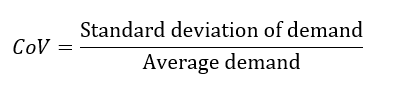
Coefficient of variability
The most common method of classifying items based on demand variability is to use the coefficient of variability:
According to your portfolio of articles you can therefore calculate the coefficients of variability and establish variability families. For each family, a suitable variability factor is assigned. In Intuiflow, this process is done through a stock buffer profiling wizard, which allows you to set up relevant stock settings for thousands of items in a few seconds.
We recommend that this CoV calculation be done based on daily demand buckets, as it is on a daily basis, given today’s demand, that our planners must make decisions.
It is also possible to calculate this CoV on a weekly or monthly basis, which leads to lower values. The thresholds of the variability categories are to be adapted, but in most cases there is a strong correlation between the variability measured on a weekly or daily basis: the items with low / medium / high / very high variability will remain the same.
Highly variable items often need to be examined more closely: are there customers who place large one-time orders? Should demand spikes be excluded from the variability assessment? Are these items really to be stocked? If they really need to be stored, wouldn’t a static buffer be a better option?
The limits of the coefficients of variability
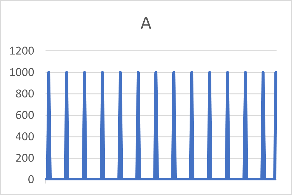
A coefficient of variability is a good basis for differentiating categories of item variability, but it does not fully characterize the demand signal.
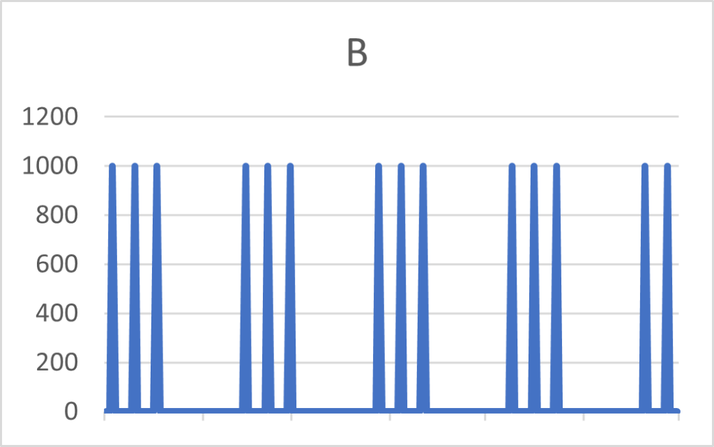
For example, the two items A and B below will have the same CoV, while their demand signals are significantly different. Depending on the replenishment lead time, item B will need a higher red zone.
Artificial intelligence and clustering
Data science techniques provide a more comprehensive approach to characterizing demand signals. As an example, the graph below shows 7 items that have similar demand signals – which is not necessarily obvious to the human eye…
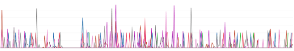
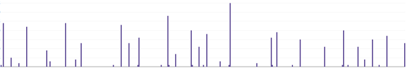
These items have CoV values between 50% and 150%, which may have led us to classify them in different variability categories, while their signals are similar.
Using the artificial intelligence approach, we can define groups of items (buffer profiles) by similarity of demand patterns and run simulations in the background to validate the red zone parameters of our dynamic buffers. The more data that feeds the machine learning engine, the better the result.
The traditional CoV approach is often a significant improvement over legacy practices, and it has the advantage of simplicity and readability. Artificial intelligence allows for a finer-grained generation of item groupings, but it must remain understandable and readable to ensure that planners can trust it.
If you want to know how Intuiflow integrates AI and Demand Driven, don’t hesitate to contact us!