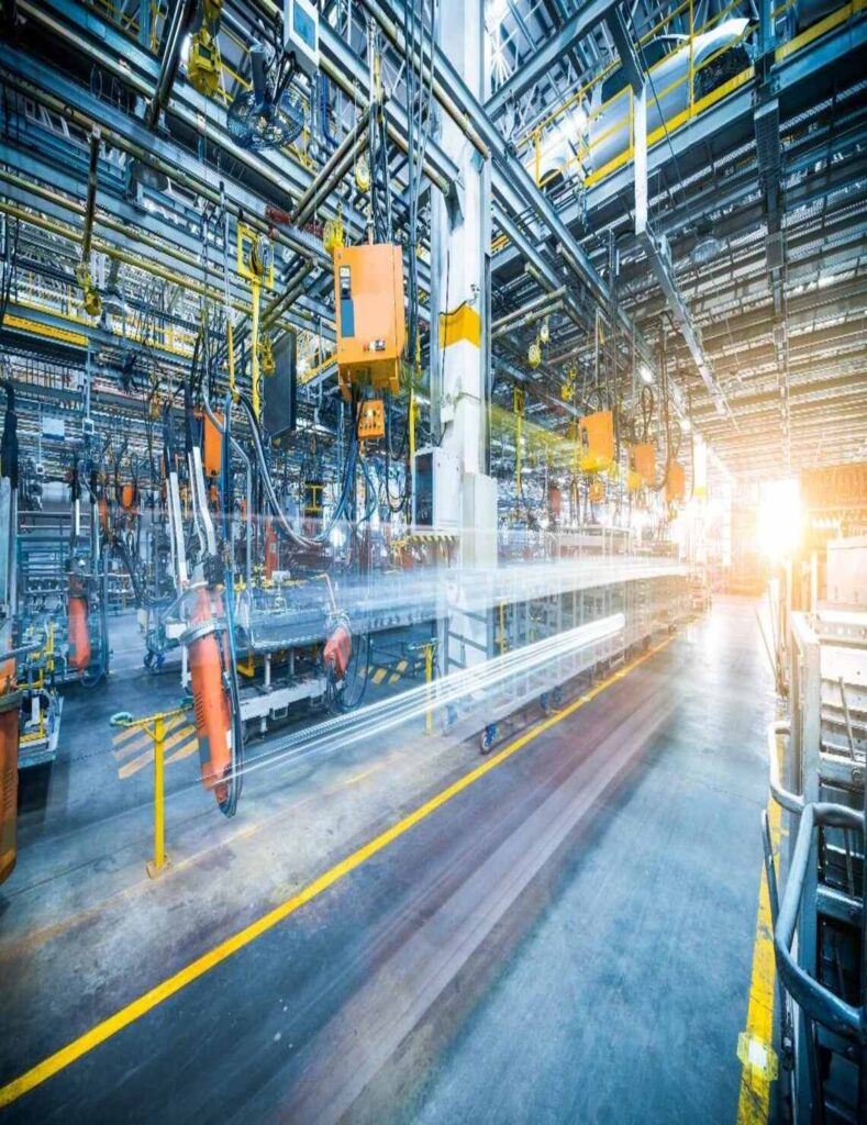
The 4.0 shop floor is about being agile, responding to real customer demand, and making priorities visible and decisions intuitive for all.
In our first article on the topic, we looked at how to start production orders at the right time. Then, we discussed how to optimize production batch size. In this article, we’ll discuss the tools that enable us to synchronize manufacturing flows with real customer demand.
Digitizing Resources and Flows
The digital revolution allows us to control our flows daily, in real time, in accordance with customer demand. The Demand Driven Operating Model (DDOM) is the methodological framework that allows us to synchronize manufacturing operations with the entire supply chain.
To manage our industrial operations daily, we need to design and represent our workshop in a computerized way. This step can be quite simple if the production operations are carried out in line, but if the flows are more complex — if the routings are made up of multiple operations calling upon common production means — the modeling will require a more complete work of analysis and collective intelligence.
Determining Flow Profiles
In a previous article, we discussed the determination of flow profiles. These profiles group together productions with similar routings. Their determination is based on analysis, for example via a VSM or via process mining, as well as on the knowledge of the production and process engineering teams.
Characterizing Production Resources
In the traditional approach to scheduling and production control software, there is a great temptation to describe everything very precisely. However, this is an illusion, because the perfect production schedule does not exist…
We therefore propose to describe the production work centers in such a way as to establish a pull-flow management mode that allows us to set unambiguous priorities and adapt to the charms of production: a few hazards here and there, a machine breakdown, a quality problem, a lower efficiency, etc.
The Three Types of Resources
We describe each production resource or resource pool under three types:
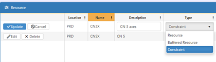
1. Constraints
A constrained resource will be loaded at finite capacity. We will finely manage its opening time and optimize the work sequence to reduce the impact of changeovers. Its demonstrated capacity will be closely monitored and will be the subject of improvement plans.
A time buffer will systematically be positioned before each constrained resource, because it is essential to ensure that they are permanently fed, since they pace the capacity of the production system.
Be careful: only define as constraints the few critical steps that are really in constraint. Too many companies try to finite capacity schedule everything, which results in terribly slowing down the flow!
There can be several constraints on a production flow; their capacity will be respected, but one of them will be defined as the leading constraint.
2. Buffered resources
These resources are not finite capacity scheduled; however, they are routing steps that must be protected by a time buffer, or that allow priorities to be handled at a key flow step. For example, we can manage the priorities of a painting installation by respecting color sequences, orchestrating subcontracted shipments, and organizing their transport in a timely fashion, etc.
In the same way that we don’t multiply constraints, we don’t multiply time buffers: they play the role of execution control points and must be limited to a few stages that deserve this attention in the daily control rituals.
3. Simple resources
These resources are not finite capacity scheduled and are not subject to time buffers. They have capacity margins, and we just must make sure, by monitoring their load, that they do not disrupt the constraints. Some companies experience “moving bottleneck” phenomena: the constraints seem to move constantly. This is often a symptom of a faulty management system — we allow occasional overloads on unconstrained resources to accumulate without reacting quickly, and these overloads end up defusing the real constraints.
An Evolving Model
Flow profiles, constraints and time buffers can change over time. For example, the product mix to be manufactured may change for a period, which modifies the load balancing. During S&OP (Sales and Operations Planning), the RCCP process (rough cut capacity planning) will surface these situations. If, for example, the system load graph shows that a resource that was previously unconstrained will be saturated for several weeks, it should be temporarily configured as constrained, and the resulting increase lead time automatically reflected in the dates promised to customers.
Monitoring of demonstrated capacity and of time buffer behavior will also fuel the evolution of this model. Don’t cast your constraints and queues in stone, so that you continuously improve the speed and stability of your flows!