The Eastern European/Central Asian market has a number of unique qualities.
Out here, the success of Western companies seems so distant from our reality that it is simply not perceived as an argument in favor of change. Western markets are more mature, according to this line of thought, and therefore more stable, predictable, and easy to work in. In addition, if you consider the financial capabilities that are required to invest in personnel development, equipment, and enterprise IT architecture, you run up against an established popular belief that most of these solutions are not relevant to post-Soviet countries.
This article was written to debunk the aforementioned myth, since most problems, as well as methods of their solution, are in fact universal and common to all continents. In reality, the more complex and unpredictable your business environment is, the greater benefit you will get from using the Demand Driven approach. I will prove this to you using the implementation of DDMRP methodology at Kormotech as an example.
Introducing Kormotech
Kormotech is a marketing and production company in the household pet care field. Founded in 2003, the company owns three high-tech cat and dog food factories in Europe and exports goods to 37 countries. In 2020, Kormotech was fifth in the world in terms of growth rate and 61st in terms of turnover, according to the top-100 household pet care companies ranking. It is a socially responsible company that seeks to change the culture of animal treatment in Eastern Europe.
Planning Before DDMRP
Before implementing DDMRP, the company demonstrated stable annual growth of about 10%. The company’s executives did not feel like there were any problems with inventory management, but they wanted to increase automation levels (i.e., avoid planning in spreadsheets), reduce stocks, and enhance the system’s transparency. At that time, their inventory management system was tuned to the traditional approach: first, the sales plan had to be developed. After that, the production plan and the purchase of raw materials would be approved based on that sales plan. Plans were updated annually, monthly, and weekly.
The traditional approach to planning assumes that if each separate function is effective, the system will be effective as a whole. For example, if we have an accurate sales plan, an optimal production plan and stock level, it will result in a high level of service and sales. Unfortunately, this statement is only true for simple linear systems, while most modern companies operate as complex and dynamic systems with many different variables. Here’s an example of a contradiction within such a system in the Kormotech company.
Production takes time. Typically, it involves the transportation and preparation of raw materials, equipment calibration and setup, production process, packaging, and preparation for shipment. In addition, both the sales plan and the requirements for efficient use of resources should be considered when performing all these operations. To ensure enough time for stable and efficient production, a weekly plan would be approved. By Friday, the company would already know what would be produced next week, down to dates and quantities.
Besides, the entire process still needed to be monitored and managed. A system of indicators was used for this purpose, including the widely used “production plan fulfillment %” indicator. At first glance, it seems that this one indicator can be used to assess two separate aspects: the system’s reliability and manageability, on one hand, and, on the other hand, its effectiveness, since the plan itself is built with production specifics considered. The higher the % of plan fulfillment is, the more predictably and efficiently production works. But what if the market demand changes and goods are wanted in a different quantity than planned? What is the planner supposed to do then? Should he ignore the plan and be ineffective, or should he produce the goods according to the plan and lose in service quality (sales), but remain “efficient” in production?
Linear perception of the system within the traditional approach suggests a simple management decision — shift the responsibility for planning accuracy to the sales and marketing department. These colleagues are supposed to know what and when we are going to sell, and production just needs to operate efficiently as clockwork. Then the whole system will be effective. But no matter how hard the sales department tries, and what software they use, their sales forecast resembles reality only at the aggregated level (month, quarter, product family, etc.). While production planning and raw materials purchase are required daily, at the level of SKU.
Mapping an Effective DDRMP Strategy
The Demand Driven method enables companies to escape this vicious circle and produce what the market really wants instead of what’s on the plan, according to your production constraints. The ABM Cloud team, together with the Kormotech team, decided to plan production daily, three days in advance. Why three days? The head of the production planning department determined this time frame to be sufficient for stable production operation, enough to complete current operations, perform preparatory work, produce the goods, as well as for subsequent work in regular mode and even with a certain extra time margin included. Why daily? Because the company’s customers place new orders every day!
At first, the idea seemed revolutionary and raised concerns that production would not be able to plan three days in advance. What if the orders suddenly peak and we simply don’t have enough time to produce the required quantity? Or vice versa. What if there is a temporary drawdown in customer orders for several days in a row? Should we just stay idle then?
The DDMRP approach teaches us that the stock, time, and power buffers are interchangeable. When we defined the buffer profiles, we considered the volume of production capacity required to compensate for demand fluctuations. On one hand, this gives us the desired stability, since the stock buffer compensates for the variability of customer orders, and production replenishes buffers according to simple and understandable priorities. And on the other hand, it brings flexibility, since production planning is based on actual customer orders (net flow balance equation), and we can be sure that we are producing what the market wants, and not what we thought we could sell.
But before we could start managing the supply chain using the DDMRP method, we had to do some preparatory work. Since previously all management work had been done via Excel, many of the parameters necessary for the automatic order generation were absent from the accounting system and we had to create the forms for maintaining data in ERP, as well as processes for entering and keeping data up to date. We have made interesting discoveries while building the new processes, and preparing for launch, some of which I will share below:
Takeaways From a DDMRP Transformation
1. Trying to minimize stocks leads to their increase.
Sounds like a paradox, doesn’t it? But what is the purchasing department’s main task? To supply the production with raw materials. In practice, this often means buying what’s listed in the monthly plan (considering current surplus, goods in transit, reserves in production, and safety stock) to meet production needs. The “A” and “B” products, which require very expensive raw materials “Х”, are not present in the next month’s production plan. Therefore, there is no point in purchasing and storing “Х” in your warehouse. If we buy it, we will worsen the turnover rate of our raw materials warehouse. Given the short delivery time of “Х” (9 days), we can purchase it as soon as we need it. We just need to wait for the product’s “A” and/or “B” to appear in the production plan.
Using DDMRP algorithms, the system has calculated buffers for the entire stored nomenclature and visualized the outcomes of such a policy from a different angle. The fact that we do not store raw materials does not mean that our customers will have to wait while we go through the purchasing and production process before we ship finished products to them. In other words, the company still stores stock, but in finished goods. You can see this in the table below.
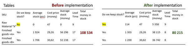
We suggested keeping a permanent stock of expensive raw materials “Х”. But since only a small amount of it is needed for producing finished goods, 115 kg in the warehouse can fully meet the production demand. Having placed a stock of raw materials “Х”, we have frozen money in raw materials. But we’ve also reduced the Lead Time of Finished goods by 9 days, which means that the stock of Finished goods can be reduced. As a result, the company has reduced the Lead Time, increased production speed and reliability while decreasing stock by 26% at the same time.
2. Trying to minimize the purchase cost leads to its increase.
Why does it happen? People tend to take the path of least resistance. If you need to reduce the cost of purchase, what is the fastest and easiest way to do it? The answer is obvious to everyone who has worked in procurement — purchase a larger batch. The more you buy, the lower the cost per unit/kilogram of raw materials. The temptation is especially great in the categories of packaging and labels. When purchasing in huge quantities, the unit price drops to 60%!
By purchasing more, you will greatly improve your cost per unit index, but it will also increase your total inventory cost. It is difficult to resist buying 100 thousand packaging items instead of the required 6 thousand, even though it will take the company 2 years to use these 100 thousand units in production… But due to constantly fluctuating sales, a 2-year stock could turn into a 3- or even 5-year stock in a few months if sales rates do not meet our current expectations.
After a few months, the company may go through rebranding, or redesign the packaging, or government requirements for packaging and labeling may change, etc. And then the rest of our profitably purchased stock will suddenly turn illiquid. This means that the cost of illiquid and low-turnover inventories, as well as the costs of their storage and future disposal, will also fall on the company’s shoulders, freezing working capital and weakening the company’s financial performance in the long term. For example, we found some dust-covered packaging tape in the warehouse. When we asked why it was there, we received a simple answer: “Someone bought it before my time.” And that employee had been working in the company for several years…
I think that the key reason why people buy large quantities cheap lies in a psychological divide between benefits and consequences. We tend to consider the benefit at the time of purchase. For example, if you buy 100 thousand units and save 60 cents per unit, that means you have just saved the company $60,000! While any consequences are likely to emerge later, sometimes in years. And sometimes, given the average staff turnover rate, it might not even be for you to clean up…
See the “Purchase batch turnover” chart for visualization of this issue.
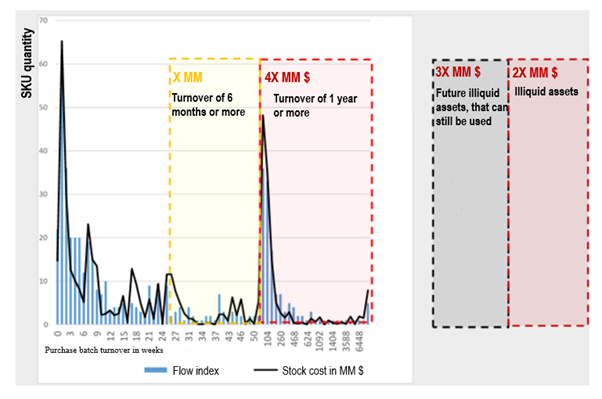
The vertical axis represents SKU quantity, the horizontal axis represents the minimum purchase batch turnover measured in weeks.
The graph shows that X million (yellow dotted line) is the turnover of the purchase batch from 6 to 12 months. 4X is the turnover of a year or more. Regardless of the inventory management method, the very fact of the purchase freezes the company’s money for years or more. This SKU category is a candidate for “future illiquid assets”. 3X million – “future illiquid assets”, are the SKUs that have no use in production, but still have a very small chance to be useful at some point in the future. And the final SKU category – 2Х million, these are illiquid assets. The remainder of the purchase batches that cannot and will not be used in production anymore. Additional costs are required for their disposal.
There is a black line on the chart — the stock cost. Its purpose is to visualize the relationship between the current cost of stock in the raw materials and packaging warehouse, and the minimum purchase batch turnover. The outlines of the black line follow the blue columns. In other words, batches with poor turnover are not only problematic as per relative indicators, but also make up a large part of the stock in monetary terms.
Less than 40% of the unique raw material SKUs were ordered during the first quarter of DDMRP method usage.
After seeing this chart, the company has revised its purchasing department target figures by limiting the sizes of purchase batches from the right side of the chart.
That is the purpose of this chart. There’s no need to revise all the purchase batches. Start at the right side of the distribution and look at the items with the lowest turnover.
3. Trying to optimize production batches leads to their imbalance them
Those of you who have performed batch optimization will confirm that after calculating an optimal batch, there is usually a general trend towards an increase in production batches. In most cases, it is readily accepted and even encouraged by production managers. I will not get into formulas for calculating the optimal batch, there are many sources on the Internet explaining different ways to achieve large production batches. I want to talk about the motivation of managers in production. I like Carol Ptak’s saying: “Tell me how you measure me, and I will tell you how I will behave.”
If you are measuring production efficiency, percentage of waste, and percentage of downtime, then there are very specific ways to influence these indicators. Usually, each launch of a specific SKU production involves a certain fixed share of losses, 100 kg for example. That’s what remains on the walls of equipment, pipes, blades, etc. Therefore, if you have produced 1000 kg of a finished product, you have 100 kg of ingredient losses, which is 10%. If you’ve produced 5000 kg of product, you will still lose 100 kg of raw material, or 2%. Note that we have just reduced production waste by 5 times! But at what cost …
Kormotech had calculated the optimal production batch, which minimized the company’s raw material losses on one hand, and on the other hand, maximized the equipment performance efficiency. A one-time production of 3000 kg for one SKU was considered optimal. The problem was that the 3-ton batch was indeed “optimal” for production, but not for the company. The sales of each item are different, but the production batch is fixed. This means that some batches will be put into production regularly, while other ones – very rarely. See the “Flow Index” chart for visualization of the “optimal” production batch turnover.
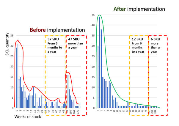
Production batch flow before and after DDMRP
The vertical axis represents SKU quantity, the horizontal axis represents the optimal production batch turnover measured in weeks.
Let’s focus on the right side of the “Before implementation” chart, which shows that 37 SKUs have a batch turnover of 6 months to a year, and 47 SKUs have a batch turnover of over a year. What does this mean for production? That they have produced the batch in one go, the percentage of losses is minimal, and let the warehouse department figure out what to do with this huge stock.
In addition to a shortage of space in the finished goods warehouse, this “optimal” production batch also led to a large-scale process of write-offs and product returns from customers. This chart raised a simple question: what’s the point of efficiently producing 3 tons of products if 1 or even 2 tons of it will end up written off. It means waste of expensive raw materials, warehouse space, operations, as well as the time of production team and equipment wear.
It became obvious that simply changing the planning procedure was not enough to solve the problem. It was necessary to completely re-evaluate the policy of optimal batches. Here is what we did:
1. We started grouping items with common semi-finished ingredients together for production purposes, since production of these ingredients was what created limitations for the system. After that, the product was packed in different sizes, which resulted in 1-3 SKUs of the finished product.
2. Instead of “optimal” batches, we started using minimal batches. The technological process was what determined their size (0.5 tons).
You can see the results of these two steps on the right side of the “After implementation” chart. Note that the number of problematic SKUs has been reduced by 4.5 times. We have freed up storage space, increased inventory turnover, and minimized returns and write-offs.
But this approach has its downside. The number of changeovers will definitely increase! If previously producing 3 tons in one go was enough for 6 months, now the product will be put in production every month, which means 5 additional changeovers in six months. If the changeover takes 1 hour, then we have increased the plant downtime by 5 hours per 6 months. And what if there’s a lot of products like that? This will both worsen the production efficiency indicators, and reduce the total volume of produced goods, which is simply unacceptable considering the constant growth of the company’s sales!
Since we sped up the slowest SKUs (by reducing their production batches), we now need to slow down the fastest ones. They can be found on the left sides of both charts, but as you can see, the “After implementation” chart has a lot more of them. To prevent this, we consider the order cycle indicator when calculating the green zone of the buffer.
3. The desired production cycle was determined to be once per every 7 days, based on the results of the production load simulation. This allowed us to compensate for the time lost in changeovers due to the reduction in slow-selling SKU batches and to improve production indicators, stabilize the production process, and, most importantly, increase the total volume of produced goods.
DDMRP Implementation Results
What are the results of a transition to DDMRP? As a result of Kormotech’s methodological and planning processes automation (which served as a foundation ensuring the sustainability of the supply chain management transformation), the following results were achieved between April and September of 2017:
1. Finished goods:
- Automated the planning process
- Increased Service Level from 90 to 99%
- Reduced overall stock level by 45% while increasing production volumes by 40%
2. Raw materials and packaging:
- Automated the planning process
- Reduced surplus by 50%
- The overall stock level remained the same, while production increased by 40%
3. Flow:
- Reduced the amplitude of fluctuations in weekly production volumes by 2.5 times
How DDMRP Impacted the Company’s Workflow
1. It reduced warehouse requirements
At the start of the project, we received a request to help justify the necessity of expanding the warehouse space. At one point before the project launch, the company was forced to temporarily stop the warehouse operation and prematurely ship a portion of the stock to distributors, since it was physically impossible to accept new items from production. By the end of the project, the need to rent additional storage space disappeared. Moreover, a lot of extra space was freed up in their warehouse. That was the impact of revising optimal batches and avoiding production plans, which became outdated faster than they could be fulfilled, with inherent errors in long-term forecasts, which were offset by the safety stocks increase.
2. It provided a single universal dashboard
Previously, there was a constant need to change the details of an already approved plan due to non-standard customer orders, or due to their absence. As a result, whatever had been planned earlier was better off not being produced at all. The production department was caught between a rock and a hard place. Produce what they ask, and it will worsen the performance indicators. Fail to produce it, and the company will lose money. “It’s hard to imagine that kind of situation today,” says the production manager. The person who plans the production sees the real market demand before anyone else, since all customer orders are visible in the planning window and that is what determines the production priority and volumes. Since everyone has the same visibility and understanding of the situation, all those letters and calls from the distribution are a thing of the past. The same goes for the raw materials and packaging stocks management. The purchasing department manager can see the real demand and any possible risks of shortage before it happens. If you can see a problem in advance, you’ll have a high chance to solve it in time.
3. It stabilized enterprise operations in the face of unstable demand
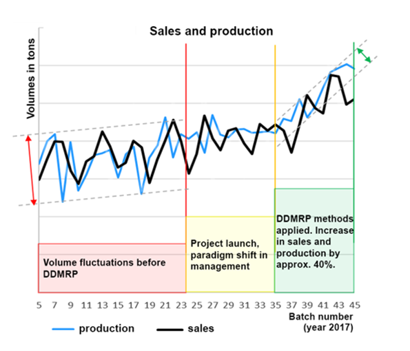
Thanks to moving away from weekly plans, the fluctuations in production volumes have also disappeared (see the “Sales and production” chart). Previously, if the weekly plan was fulfilled a little earlier, that meant we could relax at the end of the week. This can be observed in the chart at the points where the blue line (production volumes) is dropping. If this week’s production volume was smaller, then next week we would likely have to produce a lot more (but we wouldn’t know that until we got the new plan on Friday). Imagine having to plan the production process, the raw materials supply, the employee schedules, etc. in these conditions. How effective could you possibly be? As Edwards Deming used to say, if you want to improve the system’s efficiency, reduce variation. According to Deming, there are two types of variation: common cause and special cause. Common cause variation can usually be neglected, but by using traditional planning, the company exposes itself to special cause variation as well. Now look at the second part of the chart, representing the switch to DDMRP. The weekly fluctuation in output volumes decreased by 2.5 times. Imagine how much you’re planning and resource use efficiency would increase if you produce approximately the same volume of products every week.
4. It helped optimize the operational environment
Optimizing the operational environment is much easier and much more effective once the production process is stable. DDMRP also helps to digitize the effects. If, for example, you have reduced the changeover time, then you can also shorten the average order cycle, while at the same time reducing the overall stock level. DDMRP logic-based software allows you to simulate this in a few clicks and evaluate the economic effect, as well as to adapt planning and production to new conditions quickly and easily.
This project was very challenging and insightful both for the company’s management and implementation team.
It provided a great expertise, revealed weak sides of previous planning approach, opened new opportunities for the company’s development and most importantly, brought impressive effects in inventory management.